
You're not totally freaking out... not yet anyways. You know concurrency happens, which can explain why sometimes a single block Oracle read can take over a second.
But, how do you know if this is happening on your systems? How do you know if this is a problem? And, how do you easily demonstrate this to others?
The key to unlocking this mystery (and others) is the data found in v$event_histogram. And then you'll need to display it in a useful way and understand its story.
That's what this post is all about.

6ms Average Wait Time...Not The Whole Story
You may have heard about skewed data. I think it's so important for DBAs to know about this, I have blogged about it HERE and I created an online seminar entitled, Using Skewed Performance Data To Your Advantage . If you want to master this topic, you should take this seminar.
Just how easy is it to be misled and freak out? Read on...
Here's An Example Of How You Can Be Misled
Supposed you gathered 1000 sequential read wait times and 500 of the waits were 1ms, 496 of the waits were 2ms, 3 where 1000ms and the remaining sample was 2000ms. The average wait time would be 6.2ms.
For most production Oracle systems, an average single block read (wait time) of 6.2ms is not that bad. However, if I told you there were a few 1000ms reads and a 2000ms read, would that concern you? And what if over a five minute interval there were lots of 1000ms and few 2000ms reads. Would that concern you? This is when most DBAs start to freak out. But we have got to keep this in perspective.
How To Keep Perspective
In my example above the "slow" wait times occur less 5% of the time. Actually, 4% of the time. If you look at the single block read wait times on your IO intensive systems, don't be surprised if you see something similar.
If you have read books like The Black Swan or have thought about infrequent yet devastating events, you know that bad stuff can happen, just not that often.
Sometimes we care about these infrequent events, like an earthquake, a flood or a financial market crash. But sometimes, while we may care, there isn't much we can do. If so, we need to understand the risk and if necessary mitigate it.
A good example of, "there isn't much we can do" is with IO times. It is very rare for the business to invest in a 100% solid state IO subsystem or significantly alter the business workload to achieve 99.9% super fast and consistent IO times.
But before you even begin the budget discussion, we need to understand and put the "slow" IO times into perspective. A great way to better understand this type of situation is to create a histogram based on actual wait event values. Read on...
Gathering Wait Event Times To Create A Histogram
The key to unlocking this crazy single block IO time mystery is contained in the Oracle view v$event_histogram. There are other options. For example, we can manually gather the times from v$system_event or v$session. But usually, retrieving the values from v$event_histogram or DBA_HIST_EVENT_HISTOGRAM is a better solution for DBAs.
In my latest Firefighting Friday "How To" Webinar I demonstrated how to gather wait event times based on v$event_histogram resulting an series of helpful histograms. In this post, I'll do something similar.
Gathering Wait Event Times To Create A Histogram
In my OSM Toolkit there are a number of tools to gather/report Oracle wait event times. I am going to focus on gathering the data using the swEhVdGet.sql script and then copy/paste its output into the R script swEhCharts.r resulting in a magnificent two-page histogram montage. It's pretty cool.
All my wait event time SQL scripts are well documented and full of examples. Before I use them, I always check the script to remind myself of the options. If you want to really dive into this topic, I highly recommend you read the OSM event histogram readme file, osm/interactive/readmeEventHist.txt.
I created the swEhVdGet.sql script specifically so it contains no DML or DDL, and does not use DBMS_LOCK.SLEEP. Why? Because sometimes Oracle DBAs have super tight production system limitations placed on them. So, I wanted to create a script that could be simply copy and pasted directly into SQL*Plus or run from the command line.
If you look at the top of the script itself, you will notice it can be invoked a number of ways:
- Provide the parameters on the command line
- Simply run the script and have the script prompt you for the parameters
- Set the parameters and then copy and paste the script directly into SQL*Plus
Like I said, you have options!
While this script is super flexible, there is one significant downside. Because DBMS_LOCK.SLEEP is not used and I don't know of another wait to "sleep" the script, when it gathers wait times it will likely consume an entire CPU core! Ouch!
Therefore, do NOT use swEhVdGet.sql unless you have the available CPU capacity.
Thankfully, I have even more options! Take a look the OSM interactive/swEhCharts.r R script. At the top of the script, I list multiple ways to gather wait event times. But I digress...
How To Use swEhVdGet.sql
To minimize the CPU impact, the script will exit if either of these two conditions are met. First, enough samples have been collected. Second, the script has looped a specific number of times. (The looping is what consumes the CPU cycles.)
For example, suppose you want 5000 log file sync wait time samples but never want the script to loop more than 1000 times. Having the script prompt you for the parameters, do this:
SQL> @swEhVdGet
Parameter 1 is the Maximum Number Of Sampling Loops (e.g., 100)
Enter value for 1: 1000
Parameter 2 is the Minimum Number of Samples To Collect (e.g., 200)
Enter value for 2: 5000
Parameter 3 is the Wait Event Name (e.g., db%file%seq%read)
Enter value for 3: db%file%seq%read
DEFINE MAXSAMPLELOOPS  = "1000" (CHAR)
DEFINE MINSAMPLECOUNT  = "5000" (CHAR)
DEFINE ENAME           = "log%file%sync" (CHAR)

Collecting event wait times...

Copy and paste the below R code directly into the swEhCharts.r
It must be the last entry in the #2 area of swEhCharts.r

### START ###

eName = "log%file%sync"

### There were 1000 sampling loops completed and 3819 samples collected.
###
count0to1 = 0
count1to2 = 281
count2to4 = 1592
count4to8 = 1368
count8to16 = 385
count16to32 = 99
count32to64 = 68
count64to128 = 30
count128to256 = 9
count256to512 = 0
count512to1024 = 0
count1024to2048 = 0
count2048to4096 = 0
count4096to8192 = 0
count8192to16384 = 0
count16384to32768 = 0
count32768to65536 = 0
count65536to131072 = 0
count131072to262144 = 0
PL/SQL procedure successfully completed.

### END : Do NOT COPY and PASTE the "PL/SQL procedure..." TEXT INTO R ###
Next, in a text editor open the OSM R script, interactive/swEhCharts.r and scroll down to below the last example. Then copy the above output starting from the "### START ###" to just above "### END" line, being careful to NOT include the "PL/SQL..." line. Now paste that into the R script.
Next, copy and paste the entire R script directly into R. Now press ENTER and you will see two pages of carefully thought out histograms displayed before your eyes!
If you have not installed R or have never used it before, I have some resources for you!
When you paste the R script into R and press ENTER, R will produce some basic statistics (i.e., mean and median) plus two pages of carefully crafted histograms, detailing the wait event activity. Below are the statistics followed by the histograms.
> summary(binValues)
   Min. 1st Qu.  Median    Mean 3rd Qu.    Max.
  1.000   2.851   4.127   7.379   6.928 255.900


Now you can easily create proper and beautiful Oracle wait event histograms based on v$event_histogram without any DML, DDL or using DBMS_LOCK.SLEEP.
What Are The Statistics And Histograms Telling Me?
Now that you have some statistics and some histograms, it's time to learn about the underlying data. While I'll provide some guidance, my online video seminar entitled, Using Skewed Performance Data To Your Advantage will teach you to be an expert!
Here are a few observations about the data:
- The average log file sync (LFS) time is around 7.4ms. In my experience, once the average LFS exceeds 5ms I become aware that the user experience could be impacted. It's like an indicator or a "red flag."
- The typical (median) LFS time is around 4.1ms. Therefore, 50% of the LFS wait occurrences where less than about 4.1ms. Of course this also implies, 50% of the LFS wait times are greater than 4.1ms!
- 75% of the log file sync times were less than around 6.9ms. This sometimes helps people better understand that usually the LFS times are pretty good. Visually showing people a histogram or two will help them understand what happened.
- There were a few log file sync times between 128ms and 256ms. This is where you must understand (or ask questions and inform) how import consistently good LFS wait times are to the users. Almost always, a few very long LFS wait times are OK. While no one likes them and it can make people nervous, but rarely is it worth the effort and expense to eliminate them.
-
As previously mentioned, showing people a histogram or two will help them to put a few long wait times into perspective. In fact, if you only showed them the histograms and NOT the numeric statistics, they would probably dismiss the entire investigation as a waste of time!
- Most of the log file sync times where between 2ms to 8ms.
- Surprisingly, there were no log file sync times less than 1ms. Well... perhaps not that surprising.
If you want to understand the relationship between log file sync wait times and commit times, I did some very cool research on this topic and posted the results HERE.
Summary
My hope is you can calmly investigate shockingly large wait event times. Gathering some wait event data, generating the statistics, creating some histograms and taking the time to better understand the situation does not require that much effort, but the rewards are significant indeed!
To keep this post from getting to long, I did not mention how to get historical wait event data out of the AWR table, dba_hist_event_histogram. As you may have guessed, I do have a script for that. How to use that script will be the topic of my next post. But if you can't wait until next week, just watch my this OraPub "How To" Webinar .
Enjoy your work!
Craig.


