In my last article I wrote about two super-important Oracle Time Based Analysis topics: 1) The DB Time "gap" time and 2) The "gap" time increases as CPU utilization increases.
This may lead us to believe that the "gap" time is Oracle processes sitting in the CPU run queue. But as my experiment showed, the CPU run queue time only accounts for at most 25% of the "gap" time. I was shocked too!
How I figured this out and what this means in our Oracle Database tuning work is what this article is all about.
Too Busy To Read?
This is a long and very detailed article. If you can't enjoy the read and soak it all in, here is the bottom line:
We need to be aware that when the CPU utilization is high (pushing above 75%), Oracle database time will start to significantly push beyond Oracle CPU consumption plus non idle wait time. And, a significant portion of the database time increase is OS CPU run queue time. Do NOT be surprised by this or it let it bother you. But do be aware of it and factor that into your time based analysis.
Now for the good stuff... Read on.
Seeing The DB Time Gap
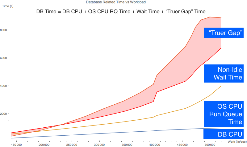
The chart to the right is based on the same experimental data that I used in my last post about the correlation between the Oracle database time "gap" time and OS CPU utilization. The massive red area is the "gap" time. Because CPU utilization correlates so strongly with the database time "gap", my hunch was that most of the "gap" time is simply the time Oracle processes are sitting in the CPU run queue. As you'll see, my hunch was totally and completely INCORRECT.
Get The Analysis Pack

You can download the Analysis Pack HERE in a single zip file. The Pack contains all my data collection scripts, the raw data, the data in an XLS spreadsheet along with all the related math, the Mathematica Notepad files that I used to the charts... everything.
What's In The DB Time "Gap?"
In theory the Oracle database time "gap" could contain a lot of things, like Oracle Database source code instrumentation error (i.e., bugs), data error from the OS (I'm not counting on this), inappropriately categorized wait event time and other things I know nothing about. I want to be clear on this; My goal is NOT to understand all the "gap" time.
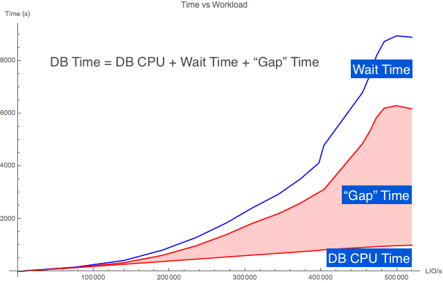
In the picture above (second from the top), the "Gap" time is shown in red. As you can see, in my experiment the "gap" time is not an insignificant part of the database time (DB time).
In this article, I want to understand how much of this "gap" time is Oracle processes sitting in the CPU run queue. That is, the time an Oracle Database foreground and background process is ready to consume OS CPU but can't because the CPUs are so busy and therefore, the process must queue. (I'm trying not to use the word wait.) So while the Oracle process is not consuming CPU, it is queued up to consume CPU.
CPU Time And The Oracle Active Session History (ASH) Facility
By the way, this OS CPU queue time is not Oracle wait time. When Oracle's Active Session History facility samples an active Oracle process that is queued to consume CPU all ASH nows is the process is not waiting and therefore "ON CPU." ASH has no idea if the process is actually consuming CPU or queued up to consume CPU. But how about Oracle's time model?
CPU Time And The Oracle Time Model
The Oracle Database Time Model (v$[sess|sys]_time_model) provides total Oracle foreground process database time (DB time) and true foreground and background process CPU consumption. If the Oracle process is a foreground process, the actual CPU consumption time is "DB CPU" and if its an Oracle background process, the actual CPU consumption time is "background cpu time".
Oracle process's gather their actual CPU consumption by calling a C function such as getrusage() or time(). We can see this by doing an OS trace on an Oracle process.
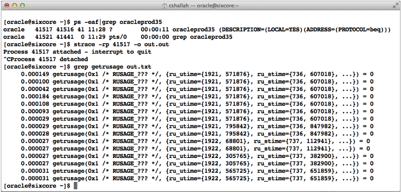
In the image to the right I used the Linux strace to capture Oracle process activity in real time. Then I grep'd out the getrusage() calls. If you look closely, you can see the Oracle process starts consuming CPU!
What Oracle time model statistics do NOT tell us is the time that an Oracle process is ready to consume CPU but can not consume CPU because the process is sitting in a CPU run queue. To figure out the CPU run queue time, we need to do a little math. And that math, is very cool math. Read on...
As Utilization Increases, So Does The CPU Run Queue
Let's remember our objective. We want to understand the relationship between the database time "gap" and the time Oracle processes are sitting in the OS CPU run queue. I'm going to show you how to figure this out, step-by-step.
When the CPU utilization increases, as some point a run queue begins to form. This is what you experience when going to lunch at the same time everyone else goes.
Some really smart guys figured out math relating work and time. Like when there are more logical IO being processed, more CPU is consumed. All DBAs know this in their gut, because we experience this relationship every day.
This math is a part of Operations Research called queuing theory. And based on some simple figures we can get from Oracle's v$ views, we can calculate/predict both the CPU run queue length and the time a process waits in the operating system CPU run queue. ...it's that cool! So, let's do this.
Calculate CPU Run Queue Time: Layout The Equation
Let's figure out the CPU run queue (RQ) time, subtract that out of the database time gap and see what is left over. I'm calling the left over gap time the, "truer gap" time.
Essentially, we want to fill in this equation with actual values:
db time  = cpu consumption time + non idle wait time + gap time
gap time = os cpu run queue time + truer gap time
db time  = cpu consumption time  + non idle wait time +
           os cpu run queue time + truer gap time
If there is no remaining or extra database time, the "truer gap" will be zero. To figure out the "truer gap" time I need to figure out the CPU run queue time. I can use basic queuing theory to figure this out. The first step is to calculate the average OS CPU utilization. Read on...
Calculate CPU Run Queue Time: Calculate CPU Utilization
It's easy to calculate the average CPU utilization. And, you can do this directly from Oracle's performance view v$OSSTAT. Because it is very important Oracle DBAs to understand and know how to calculate CPU utilization on our database servers, I have blogged about this many times HERE and dig deep into this topic in my online video seminar, Utilization On Steroids.
The inputs are the number CPU cores and the CPU utilization. On my database server there are 6 CPU cores. The most reliable and actually the easiest way to figure out CPU utilization using the busy_time and idle_time from v$osstat. This is why I collected these stats in this experiment.
To demonstrate this I'm going to use just one experimental sample and some basic queuing theory. I will use the sample where the load_no is 13 and the sample number is 18. For this sample, the busy_time is 92305 cs (column I) and the idle_time is 15684 cs (column J) therefore the average CPU utilization over the 180 second experimental sample interval is 0.85 that is, 85%. (Column P) 0.8548=92305/(92305+15684)
Calculate CPU Run Queue Time: Calculate CPU Service Time
Remember, our objective is to determine the CPU run queue time. According to the queuing theory (see my book, Forecasting Oracle Performance ), CPU utilization equals:
U = ( St * L ) / M
where:
St is the service time. This is how long it takes to process a transaction with no queuing. This is also our unknown variable.
L is the arrival rate. This is the total workload divided by the snapshot interval.
M is the number of CPU cores, which in this case is six.
Now, let's do a little Algebra to solve for the service time.
St = U*M/L
Now let's put our actual experimental data into the formula. You can see the data in the analysis spreadsheet columns N to V.
St = 0.8548 * 6 / (82140393 LIO / 180.03 seconds)
   = 5.129 / 456259 seconds/LIO
   = 0.00001124 seconds/LIO
   = 0.0112 ms/LIO
During the sample interval, the average service time was 0.0112 ms/LIO. You can see how I did this in the spreadsheet in column S. The next step is to figure out the response time. Read on...
Calculate CPU Run Queue Time: Calculate CPU Response Time
Response time is how long it takes to process a single piece of work, like a transaction. Response time always includes some service time and may contain some queue time. Before we can figure out the CPU queue time, we need to figure out the CPU response time. The response time formula (there are others) for a CPU subsystem is shown in the analysis spreadsheet column T and shown below:
Rt = St / (1-U^M)

   = 0.0112 ms/LIO / (1-0.8548^6)
   = 0.0112 ms/LIO / 0.6099
   = 0.0184 ms/LIO
So, over the sample interval, on average, it took 0.0184 ms to process a single LIO.
Extra credit: Notice in the above formula, that as the utilization (U) increases, so does the response time. And when the utilization is low, the response time will equal the service time!
Now we're ready to calculate the CPU run queue time. Read on...
Calculate CPU Run Queue Time: Per LIO
Since we know the service time plus the queue time equals the response time,
Rt = St + Qt
then
Qt = Rt - St
   = 0.0184 ms/LIO - 0.0112 ms/LIO
   = 0.0072 ms/LIO
You can see this math detailed in the analysis spreadsheet column U. So, over the sample interval and on average, a processes was in the CPU run queue for 0.0072 ms while processing a single LIO.
Extra credit: Notice in the above formula, when the service time equals the response time, the queue time is zero!
Calculate CPU Run Queue Time: All CPU Run Queue Time
For our experimental sample, the average CPU run queue time is 0.0072 ms/LIO. This is important: This represents the queue time for a single LIO being processed... and during a sample interval there were LOTS AND LOTS of LIOs being processed.
During this particular sample interval, there were 82140393 LIOs processed. This means the total CPU run queue time is the sum of the queue time for each LIO processed. You can see this detailed in the analysis spreadsheet column V, which contains more significant digits. Here's the math:
Total Qt = Qt * LIO
         = 0.0072 ms/LIO * 82140393 LIO
         = 591410.83 ms
         = 591.4 seconds
So, during our sample interval and on average during the processing of all the LIOs, Oracle processes where in the CPU run queue for a total of 591.4 seconds!
This 591.4 seconds of CPU run queue time is part of database time. But it is not Oracle process CPU consumption (DB CPU or background cpu time) and is not non-idle wait time. Therefore, it must be part of the database "gap" time.
Side Note: If you are intrigued by the above process and want to build robust forecasting models to answer questions like, When will our database server "run out of gas?" than check out my upcoming Oracle Forecasting & Predictive Analysis class in Florida this June. It will be HOT!
The "Truer" DB Time Gap For Our Single Sample
Now it's time to put the pieces or classifications of time together. Our original equation is:
db time = cpu consumption + non idle wait time + gap
But we know the CPU run queue time and that is is part of the "gap" time:
gap = cpu run queue time + truer gap
I call the remaining "gap" time the truer gap time because we have a better understanding of the gap time. Now, let's put this all together:
db time = cpu consumption + non idle wait time + cpu run queue time + truer gap
It's time to solve for the "truer gap", which is:
gap       = db time    - db cpu    - niwt
          = 6776.8 sec - 910.7 sec - 1917.4 sec
          = 3948.7 sec

truer_gap = db time    - db cpu    - ni wait time - cpu rq time
          = 6776.8 sec - 910.7 sec - 1917.4 sec   - 591.4 sec
          = 3355.4 sec
So, in our one example the CPU run queue time only accounted for 14% of the gap (which, by the way is really disappointing).
Truer Gap % = 1 - truer_gap / gap
            = 1 - 3355.4 sec / 3948.7 sec
            = 1 - 0.850
            = 0.15
            = 15%
I think it's difficult to get a sense for the above 15%. Sure, the original "gap" time is 3948.7 seconds and the CPU run queue time is 591.4 seconds, reducing the "gap" to a "truer gap" time of 3355.4 seconds. But in working you through this process, I used only one experimental sample. To better understand the "truer gap" and the role of OS CPU run queue time in Oracle database time we need to look at all the samples. That's what I'm doing next. Read on...
The "Truer" DB Time Gap For The Entire Experiment
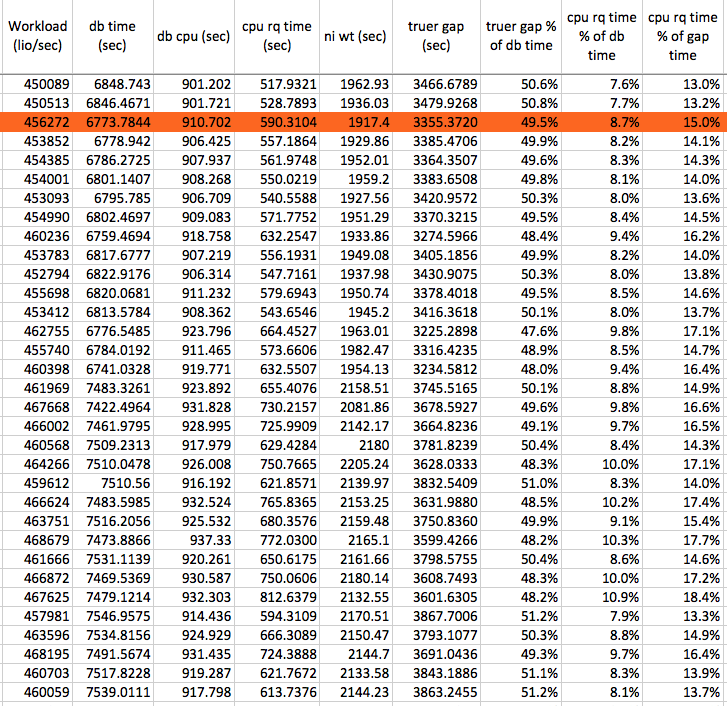
To better understand the "truer gap" and the role of OS CPU run queue time, I analyzed all the experimental samples. The data for the chart below has the same source as the analysis spreadsheet columns Z to AG. The row highlighted in red is the example sample I have been using throughout this article.
Since I have lots of samples and at different workloads, I created a chart showing the above database time components on the vertical axis in relation to the workload intensity shown on the horizontal axis. Here is the resulting chart.

It's pretty easy to tell from the above chart that very-roughly around 50% of the "gap" time ("truer gap" plus CPU RQ time) was filled with CPU run queue time.
In fact, if you look at the values (column AF) in the analysis spreadsheet you will see the "truer" gap time accounts from around 40% to 50% of the database time and the CPU run queue time accounts (column AG) from 1% to 14% of the database time. The reason for the increasingly large percentage spread is because as the workload increases, so does the CPU utilization and therefore so does the CPU run queue time.
To summarize, while CPU run queue time significantly reduced the "gap" time, the are other factors contributing to the "gap" time. In other words, while the CPU run queue time is a big part of the "gap" time it is not even close to being most of it.
The Take-Aways: Read This First
My experiment demonstrated a situation where the Oracle database time did not equal all the Oracle foreground process CPU consumption plus all the non idle wait time. The objective of my experiment was to better understand this time difference ("gap" time) and to understand how OS CPU run queue time was involved.
Below are some key take-aways:
- Oracle database time does not always equal all the Oracle foreground process CPU consumption (DB CPU) plus the non idle wait time. I call this the database time "gap". You can easily see this in the analysis spreadsheet, column K ("Gap").
- As CPU utilization increases, so does this database time "gap." I demonstrated this in my prior article and this can be seen in the analysis spreadsheet columns, K ("Gap") and P (Utilization).
- As the LIO workload increased, so did the CPU utilization, columns O (workload) and P (utilization). Even better is columns R (arrival rate) and P (utilization).
- As the CPU utilization increased, so did the CPU run queue time. Columns P (utilization) and U (Qt).
- The CPU run queue time accounts for around 1% to 25% of the database time "gap" time. Columns AH (cpu rq time % of gap time).
- The CPU run queue time accounts for around 1% to 14% of the database time. Columns AG (cpu rq time % of db time).
- I did not explore the time related to the "truer" gap time. It could be time related to Oracle Database source code instrumentation error (i.e., bugs), data error from the OS (I'm not counting on this), inappropriately categorized wait event time and other things I know nothing about.
The Big Take Away: What Does This Mean For A DB Time Based Analysis?
I think the entire experiment can be distilled down to this:
We need to be aware that when the CPU utilization is high (pushing above 75%) Oracle database time will start to significantly push beyond Oracle CPU consumption plus non idle wait time. And, a significant portion of the database time increase is OS CPU run queue time. Do NOT be surprised by this or it let it bother you. But do be aware of it and factor that into your time based analysis.
It's important to keep in mind that my experiment is just one experiment. And it's an experiment where I purposely and forcefully placed an Oracle logical IO workload on the system to increase the CPU utilization. So do NOT expect your systems to look just like my experimental system.
I hope you enjoyed this article. It took me a tremendous of time and effort to put it together.
Thanks for reading!
Craig.


